EconomicScenarioGenerators.jl

Note

Maintenance mode. For single-model interest-rate scenario generation, prefer FinanceModels.ShortRate.{Vasicek, CoxIngersollRoss, HullWhite} together with FinanceModels.simulate/pv_mc (FinanceModels ≥ 6), which are the maintained successors of this package's generators. EconomicScenarioGenerators.jl remains the home of Correlated — copula-correlated simulation across multiple models — which FinanceModels does not provide. Bug fixes continue; new features land in FinanceModels.

Interested in developing economic scenario generators in Julia? Consider contributing to FinanceModels.jl. Open an issue, create a pull request, or discuss on the Julia Zulip's #actuary channel.

Usage

EconomicScenarioGenerators.jl is available via the General Registry. Install and use in the normal way:

1. Add EconomicScenarioGenerators via Pkg
2. import EconomicScenarioGenerators or using EconomicScenarioGenerators in your code

Examples

Importing packages

First, import both EconomicScenarioGenerators and FinanceModels:

using EconomicScenarioGenerators
using FinanceModels

Models

Interest Rate Models

• Vasicek
• CoxIngersollRoss
• HullWhite

EquityModels

• BlackScholesMerton

Interest Rate Model Examples

Vasicek

m = Vasicek(0.136,0.0168,0.0119,Continuous(0.01)) # a, b, σ, initial Rate
s = ScenarioGenerator(
        1,  # timestep
        30, # projection horizon
        m,  # model
    )

You can collect a single generated scenario like so:

rates = collect(s)

And the package integrates with FinanceModels.jl:

YieldCurve(s)

will produce a yield curve object (if UnicodePlots.jl has also been imported):

              ⠀⠀⠀⠀⠀⠀⠀⠀⠀⠀⠀Yield Curve (FinanceModels.Yield.Spline)⠀⠀⠀⠀⠀⠀⠀⠀⠀⠀⠀           
              ┌────────────────────────────────────────────────────────────┐           
         0.04 │⠀⠀⠀⠀⠀⠀⠀⠀⠀⠀⠀⠀⠀⠀⠀⠀⠀⠀⠀⠀⠀⠀⠀⠀⠀⠀⠀⠀⠀⠀⠀⠀⠀⠀⠀⠀⠀⠀⠀⠀⠀⠀⠀⠀⠀⠀⠀⠀⠀⠀⠀⠀⠀⠀⠀⠀⠀⠀⠀⠀│ Zero rates
              │⠀⠀⠀⠀⠀⠀⠀⠀⠀⠀⠀⠀⠀⠀⠀⠀⠀⠀⠀⠀⠀⠀⠀⠀⠀⠀⠀⠀⠀⠀⠀⠀⠀⠀⠀⠀⠀⠀⠀⠀⠀⠀⠀⠀⠀⠀⠀⠀⠀⠀⠀⠀⠀⠀⠀⠀⠀⠀⠀⠀│           
              │⠀⠀⠀⠀⠀⠀⠀⠀⡀⠀⠀⠀⠀⠀⠀⠀⠀⠀⠀⠀⠀⠀⠀⠀⠀⠀⠀⠀⠀⠀⠀⠀⠀⠀⠀⠀⠀⠀⠀⠀⠀⠀⠀⠀⠀⠀⠀⠀⠀⠀⠀⠀⠀⠀⠀⠀⠀⠀⠀⠀│           
              │⠀⠀⠀⠀⠀⠀⡠⠎⠉⠉⠊⠉⠑⠦⠤⠤⣄⡀⠀⠀⠀⠀⠀⠀⠀⠀⠀⠀⠀⠀⠀⠀⠀⠀⠀⠀⠀⠀⠀⠀⠀⠀⠀⠀⠀⠀⠀⠀⠀⠀⠀⠀⠀⠀⣀⣀⡠⠤⠤⠔│           
              │⠀⠀⠀⠀⢀⠖⠁⠀⠀⠀⠀⠀⠀⠀⠀⠀⠀⠉⠑⠦⢄⣀⠀⠀⠀⠀⠀⠀⠀⠀⠀⠀⠀⠀⠀⠀⠀⠀⠀⠀⠀⠀⠀⠀⢀⣀⣀⣀⠤⠔⠒⠊⠉⠉⠀⠀⠀⠀⠀⠀│           
              │⠀⠀⠀⢰⠃⠀⠀⠀⠀⠀⠀⠀⠀⠀⠀⠀⠀⠀⠀⠀⠀⠀⠉⠓⠒⠦⠤⢄⣀⠀⠀⠀⠀⠀⠀⠀⠀⣀⣀⠤⠔⠒⠉⠉⠁⠀⠀⠀⠀⠀⠀⠀⠀⠀⠀⠀⠀⠀⠀⠀│           
              │⠀⠀⠀⡎⠀⠀⠀⠀⠀⠀⠀⠀⠀⠀⠀⠀⠀⠀⠀⠀⠀⠀⠀⠀⠀⠀⠀⠀⠀⠉⠒⠒⠒⠒⠊⠉⠉⠁⠀⠀⠀⠀⠀⠀⠀⠀⠀⠀⠀⠀⠀⠀⠀⠀⠀⠀⠀⠀⠀⠀│           
   Continuous │⠀⠀⢰⠁⠀⠀⠀⠀⠀⠀⠀⠀⠀⠀⠀⠀⠀⠀⠀⠀⠀⠀⠀⠀⠀⠀⠀⠀⠀⠀⠀⠀⠀⠀⠀⠀⠀⠀⠀⠀⠀⠀⠀⠀⠀⠀⠀⠀⠀⠀⠀⠀⠀⠀⠀⠀⠀⠀⠀⠀│           
              │⠀⠀⡇⠀⠀⠀⠀⠀⠀⠀⠀⠀⠀⠀⠀⠀⠀⠀⠀⠀⠀⠀⠀⠀⠀⠀⠀⠀⠀⠀⠀⠀⠀⠀⠀⠀⠀⠀⠀⠀⠀⠀⠀⠀⠀⠀⠀⠀⠀⠀⠀⠀⠀⠀⠀⠀⠀⠀⠀⠀│           
              │⠀⡸⠁⠀⠀⠀⠀⠀⠀⠀⠀⠀⠀⠀⠀⠀⠀⠀⠀⠀⠀⠀⠀⠀⠀⠀⠀⠀⠀⠀⠀⠀⠀⠀⠀⠀⠀⠀⠀⠀⠀⠀⠀⠀⠀⠀⠀⠀⠀⠀⠀⠀⠀⠀⠀⠀⠀⠀⠀⠀│           
              │⢀⡇⠀⠀⠀⠀⠀⠀⠀⠀⠀⠀⠀⠀⠀⠀⠀⠀⠀⠀⠀⠀⠀⠀⠀⠀⠀⠀⠀⠀⠀⠀⠀⠀⠀⠀⠀⠀⠀⠀⠀⠀⠀⠀⠀⠀⠀⠀⠀⠀⠀⠀⠀⠀⠀⠀⠀⠀⠀⠀│           
              │⡸⠀⠀⠀⠀⠀⠀⠀⠀⠀⠀⠀⠀⠀⠀⠀⠀⠀⠀⠀⠀⠀⠀⠀⠀⠀⠀⠀⠀⠀⠀⠀⠀⠀⠀⠀⠀⠀⠀⠀⠀⠀⠀⠀⠀⠀⠀⠀⠀⠀⠀⠀⠀⠀⠀⠀⠀⠀⠀⠀│           
              │⠉⠉⠉⠉⠉⠉⠉⠉⠉⠉⠉⠉⠉⠉⠉⠉⠉⠉⠉⠉⠉⠉⠉⠉⠉⠉⠉⠉⠉⠉⠉⠉⠉⠉⠉⠉⠉⠉⠉⠉⠉⠉⠉⠉⠉⠉⠉⠉⠉⠉⠉⠉⠉⠉⠉⠉⠉⠉⠉⠉│           
              │⠀⠀⠀⠀⠀⠀⠀⠀⠀⠀⠀⠀⠀⠀⠀⠀⠀⠀⠀⠀⠀⠀⠀⠀⠀⠀⠀⠀⠀⠀⠀⠀⠀⠀⠀⠀⠀⠀⠀⠀⠀⠀⠀⠀⠀⠀⠀⠀⠀⠀⠀⠀⠀⠀⠀⠀⠀⠀⠀⠀│           
        -0.01 │⠀⠀⠀⠀⠀⠀⠀⠀⠀⠀⠀⠀⠀⠀⠀⠀⠀⠀⠀⠀⠀⠀⠀⠀⠀⠀⠀⠀⠀⠀⠀⠀⠀⠀⠀⠀⠀⠀⠀⠀⠀⠀⠀⠀⠀⠀⠀⠀⠀⠀⠀⠀⠀⠀⠀⠀⠀⠀⠀⠀│           
              └────────────────────────────────────────────────────────────┘           
              ⠀0⠀⠀⠀⠀⠀⠀⠀⠀⠀⠀⠀⠀⠀⠀⠀⠀⠀⠀⠀⠀⠀⠀⠀⠀⠀⠀time⠀⠀⠀⠀⠀⠀⠀⠀⠀⠀⠀⠀⠀⠀⠀⠀⠀⠀⠀⠀⠀⠀⠀⠀⠀⠀⠀30⠀        

CoxIngersollRoss

A CIR model:

m = CoxIngersollRoss(0.136,0.0168,0.0119,Continuous(0.01))

Hull White Model using a FinanceModels.jl yield curve

Construct a yield curve and use that as the arbitrage-free forward curve within the Hull-White model.

using FinanceModels, EconomicScenarioGenerators
rates = [0.01, 0.01, 0.03, 0.05, 0.07, 0.16, 0.35, 0.92, 1.40, 1.74, 2.31, 2.41] ./ 100
mats = [1 / 12, 2 / 12, 3 / 12, 6 / 12, 1, 2, 3, 5, 7, 10, 20, 30]
c = FinanceModels.fit(
    FinanceModels.Spline.Cubic(),
    FinanceModels.ZCBYield.(rates, mats),
    FinanceModels.Fit.Bootstrap()
)

m = HullWhite(2.0, 0.025, c)

s = EconomicScenarioGenerators.ScenarioGenerator(
    0.01,                              # timestep
    30.0,                             # projection horizon
    m
)

Create 1000 yield curves from the scenario generator:

n = 1000
curves = [YieldCurve(s) for i in 1:n]

Plot the result:

using CairoMakie

times = 1:30

fig = Figure()
axis = Axis(fig[1,1],title="EconomicScenarioGenerators.jl Hull White Model",xlabel="time",ylabel="rate")
# plot the zero rates
for d in curves
    lines!(axis,times,rate.(zero.(d,times)),alpha=0.1,label="")
end
lines!(axis,times,rate.(zero.(c,times)),color=:black,linewidth=7)
fig

Equity Model Examples

BlackScholesMerton

m = BlackScholesMerton(0.01,0.02,.15,100.)

s = ScenarioGenerator(
               1,  # timestep
               30, # projection horizon
               m,  # model
           )

Instantiate an array of the projection with collect(s).

Plotted BSM Example

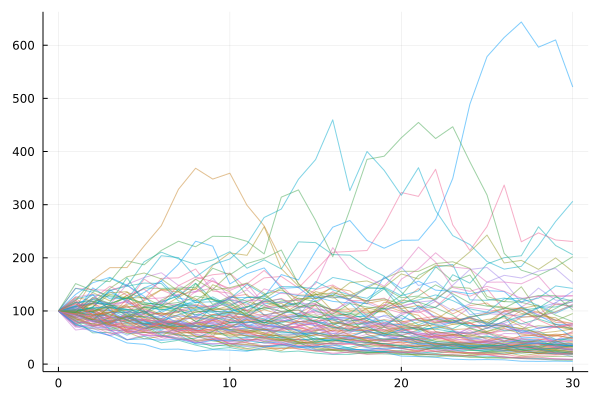
Plot 100 paths:

using Plots
projections = [collect(s) for _ in 1:100]

p = plot()

for p in projections
    plot!(0:30,p,label="",alpha=0.5)
end

p

Correlated Scenarios

Combined with using Copulas, you can create correlated scenarios with a given copula. See ?Correlated for the docstring on creating a correlated set of scenario generators.

Example

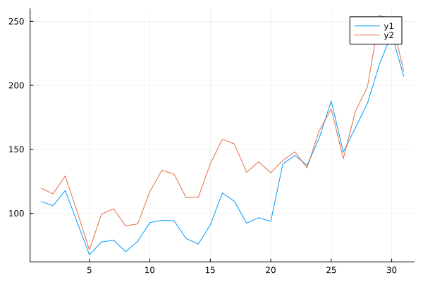
Create two equity paths that are 90% correlated:

using EconomicScenarioGenerators, Copulas

m = BlackScholesMerton(0.01,0.02,.15,100.)
s = ScenarioGenerator(
                      1,  # timestep
                      30, # projection horizon
                      m,  # model
                  )

ss = [s,s] # these don't have to be the exact same, but do need same shape
g = ClaytonCopula(2,7) # highly dependent model
c = Correlated(ss,g)

x = collect(c) # an array of tuples

using Plots

# get the 1st/2nd value from the scenario points
plot(getindex.(x,1))
plot!(getindex.(x,2))

Other ESG packages

• Python
  • https://github.com/jason-ash/pyesg